
Power Meter - Calibration
For proper operation of the Microwave Power Meter, a calibration system was developed, working as a dynamic mapping function that converts the Power Meter Probe voltage to the corresponding input power.
The calibration system and procedures determines the final absolute accuracy of the equipment, and its design needs to allow for the wanted final specifications.

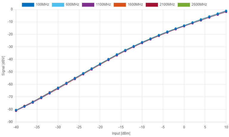
The probe response behaves different for changes of input frequency. In the upper figure, we have seven responses across the input range. Even being almost identical, these slight differences produce inaccuracies 10x higher than the goal of 0.3dB.
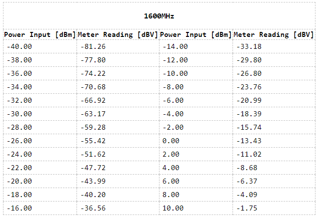
The first step for calibration is the capture of the data points. The input amplitude range was divided in steps of 2dB and frequency range in steps of 100MHz. A full sweep from -40dBm to 10dBm was taken for each frequency step, covering the 100MHz - 3GHz operational range.
This characterization process was automated using a E4421 signal generator with GPIB and the power meter streaming its raw voltage measurement by serial over USB. A JavaScript NodeJS application sweeps the RF amplitude and frequency, while recording the measured voltage.
The main difficult on the design of the calibration subsystem was the available EEPROM memory on the ATMega328 microcontroller. With the 1024 bytes of non-volatile memory, there was no possibility of recording the raw date directly. A quick calculation shows that, with 26 amplitude steps (-40 to 10dBm in 2dB increments) at 30 different frequencies, using floating points (4 bytes), the minimum requirement would be 3120 bytes!
Data compression
A fast and simple data compression scheme was designed, allowing the full calibration data to fit in memory with margin.
The compression first calculates the average response for all input frequencies, generating a base curve. This curve is written to memory in floating-point, using 4 bytes for each amplitude step, consuming a total of 104 bytes.
For each frequency step, the difference between the actual response and the base is taken, resulting in correction factors in respect to the average response. These corrections terms are small, as each frequency response is only slightly different.
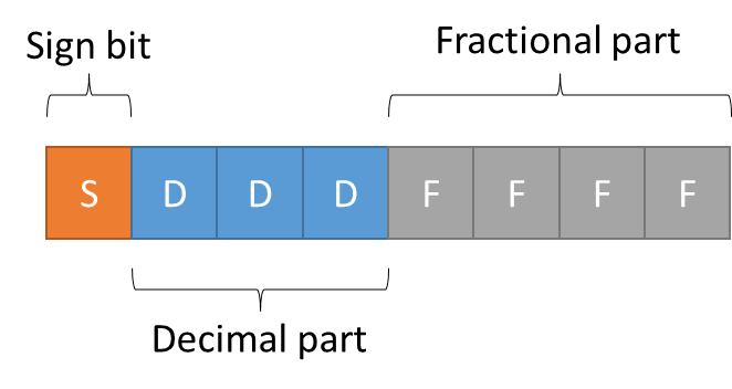
Each correction term is then converted to a fixed-point format, using only one byte. The MSB is used to encode the sign of the correction, 3 bits are used for the decimal part and 4 bits for the fractional part. This allows the encoding of the correction with enough precision to accomplish the 0.3dB accuracy wanted for the project.
Linear interpolation is done for voltage readings that are in between data points.
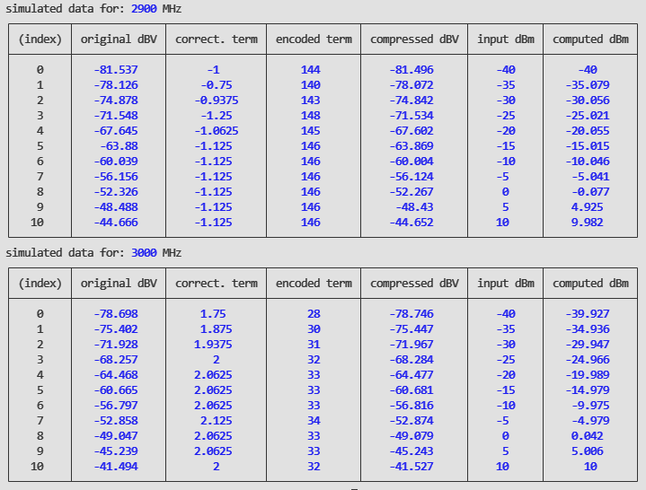
This simulation was done using real data grabbed from the probe by the automation setup. We see that the measured dBV values differs for the 2900MHz and 3000MHz. The correction terms are calculated for each amplitude step and encoded in the fixed-point format. These results show us that the scheme is able to compute the correct input power with better than 0.1dB accuracy.
The calibration data I have for two probes I constructed don't show correction terms higher than 3 in magnitude, suggesting that an SDDFFFFF encoding could provide more fractional resolution for the compressed dBV values. This theoretical increase would not reflect in practical results, as the 0.3dB goal covers inaccuracies in the overall system.
When a frequency is selected on the power meter LCD that is not exactly represented by calibration data points, two curves, lower and higher in frequency, are used. The two tables are decompressed from memory, the conversion is computed from the two curves and a linear interpolation is done between the readings.
The final memory usage is 26 * 4 bytes for the average response + 1 byte for each amplitude step in each frequency step. This results in only 884 bytes, 28% of the initial figure!