A Simple 2nd Order Low-Pass Filter
Usually, when developing signal processing applications, we encounter the need for low-pass filtering - for reducing noise in sampled systems, averaging sensor measurements or, as will be discussed at the end of the article, for closed-loop controllers that use derivative gain.
The architecture presented here implements a second-order low-pass structure, by placing a pair of complex poles in the Z-plane. Controlling the poles' radius and angle allows the designer to configure the filter for the required resonance frequency and Q factor.
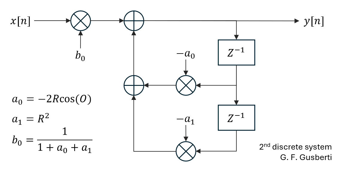
Two delay units are used in direct-form I [1], the coefficients are derived from the poles' positions and can be pre-calculated to reduce the number of real-time computations. The unique feedforward term b0 can be used to compensate for the DC gain, normalizing the transfer function to 0 dB at 0 Hz.
A simple transfer function with a pair of conjugate poles defined by radius R and angle O, in the form 1 / [(1 - R × ejω × Z-1)(1 - R × e-jω × Z-1)], can be expressed as a second-order transfer function 1 / [1 - 2 × R × cos(O) × Z-1 + R2 × Z-2]. The factors 2 × R × cos(O) and R2 are the factors a0 and a1 of the filter [2].
The design of the filter can be performed in the continuous time-domain, by carefully choosing the position of the poles in the S-plane, based on the design requirements. As the architecture doesn't have any zero - just the two conjugate poles - the poles can be transferred to the Z-plane by the usage of the impulse-invariance technique.
By thinking about the filter in the S-plane, it allows for the designer to have common 2nd-order continuous-time transfer-function parameters as the input. For example, the filter designed in this article will be a function of the resonance frequency - the damped frequency ωd - and the damping factor ξ.
Engineers usually think in terms of the quality factor Q and not much about damping ξ. For a 2nd-order system, both are related by Q = 1 / 2ξ, making it possible to have Q as the design input.
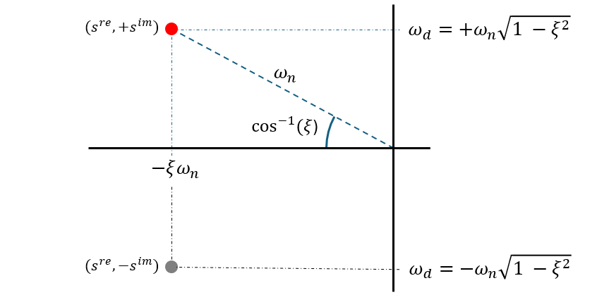
The design starts by positioning a positive-frequency pole in the S-plane, by using the pole's geometrical properties for a 2nd-order system. It is implicit that the negative-frequency pole is being positioned in simultaneous (because they form a conjugate pair).
For this example, the design constraints will be the resonance frequency Fr (in Hz), and the damping factor ξ, that will be represented by the letter variable Z. In Figure 2 we see that the pole's radius length is its natural frequency ωn, and the angle is a function of the damping.
This location in the S-plane results in projections into the real and imaginary axes, where the real axis length is -ωn × ξ, and the imaginary axis length is the damped frequency ωd = ωn × sqrt(1 - ξ2).
We start by fixing the damped frequency ωd using the required resonance Fr, by setting ωd = 2 × pi × Fr - this results directly in the imaginary component sim for the s pole (as seen in Figure 2). Following the geometry, the real part sre is found by ωd × Z / sqrt(1 - Z2).
Using a fixed ωd is an unusual way of design, but it is useful for engineering purposes, as usually the resonance peak is the point of interest. Nevertheless, the reader can choose different input constraints, adjusting the pole positioning accordantly.
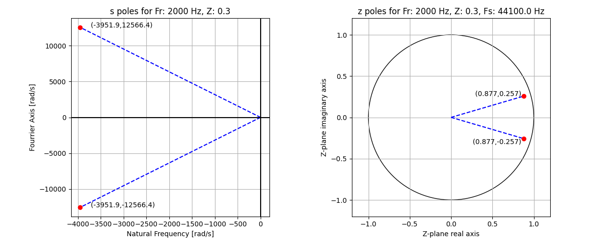
To transform the filter to discrete domain, the S-poles must be mapped to the Z-plane. Each continuous-time pole si is mapped to a discrete-time pole zi by the relationship zi = esiT, with T being the sampling interval of the discrete-time model. This creates the special condition where the impulse response of the digital model is equal to a sampled version of the impulse response of the continuous system [3].
Impulse invariance does not guarantee that the frequency response of the discrete system will be equal to the original continuous-time system [4]. However, it leads to a good first approximation that can be tweaked manually by the designer if needed.
Again, as the discrete transfer function chosen presents a pair of conjugate poles - with radius R and angle O - it is necessary to just think about the positive-frequency pole. The radius of the mapped z pole becomes R and its angle becomes O, thus being applied directly in the architecture of the filter.
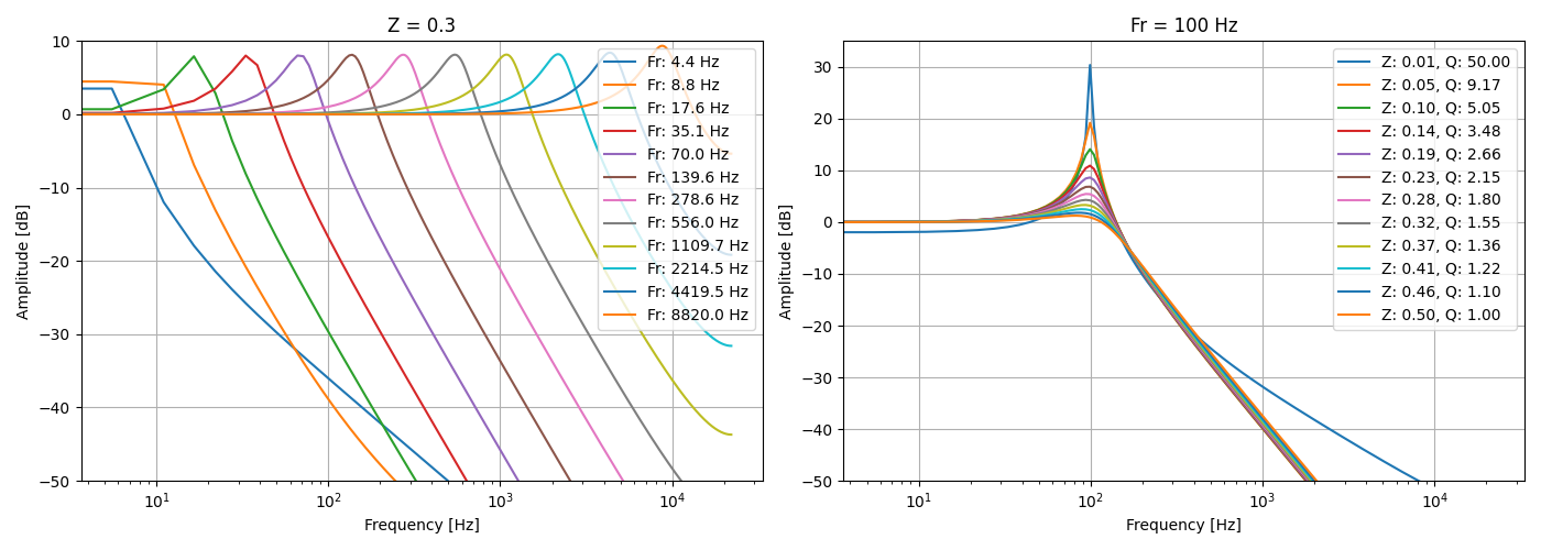
In Figure 4 it is possible to see a sweep of the design parameters. At the left, the filters have different resonant frequencies and constant damping. On the right side, the resonant frequency is kept constant, and the damping factor is swept.
The proposed architecture is implemented as a simple difference equation. All the plots in Figure 4 were generated by iterating the filter for a unity-impulse input at t0 (first sample), generating the filter's impulse response at the output. Computing the FFT of the impulse response generates the frequency response, that is shown on the graphs.
# Gusberti Analog @ 2024
# Visit https://youtube.com/allelectronicschannel
# Developed by G. F. Gusberti

def calc_filter(freq_resonance, damping, Ts):
    Fr = freq_resonance
    Z  = damping

    # we could have defined the filter by
    # its Q factor and not damping Z.
    Q  = 1 / (2 * Z)     # this will be the quality factor

    # the calculation is done by a single pole
    # because the fact that the poles are a conjugate pair
    # is implicit in the choice of transfer function / difference
    # equation.

    # place the damped frequency Wd (resonance) at the desired position.
    sp_j = 2 * math.pi * Fr
     # find natural frequency Wn, it is the projection in the real axis.
    sp_r = -sp_j * Z / math.sqrt(1 - Z**2)
    sp   = sp_r + sp_j * 1j    # makes the complex pole.
    zp   = cmath.exp(sp * Ts)  # move it to z-plane using impulse invariance.

    print(Z, abs(sp), cmath.phase(sp))

    # the difference equation we are using required the
    # angle and radius of the poles in the z-plane.
    zp_a = cmath.phase(zp)     # angle in the z-plane
    zp_R = abs(zp)             # radius in the z-plane

    # gain at DC is calculated by evaluating the
    # transfer function at 0 Hz.
    G  = 1 / (1 - 2 * zp_R * math.cos(zp_a) + zp_R**2)

    z1 = 0
    z2 = 0
    y_vec = []
    x_vec = []

    N = 5000
    for i in range(N):
        x = 1 / G if i == t else 0
        y = x + z1 * 2 * zp_R * math.cos(zp_a) - zp_R**2 * z2
        x_vec.append(x)
        y_vec.append(y)
        z2 = z1
        z1 = y

    y_fft = spec(y_vec)
    y_phs = phase(y_vec)
    x_fft = np.linspace(0, 0.5 / TS, len(y_fft))

    return x_vec, y_vec, x_fft, y_fft, y_phs, sp, zp
Low-Pass Derivative
Control applications that require derivative action - as in the case of the PID controller, for example - require that the derivator presents a low-pass behavior outside the frequencies of interest. This is needed because a pure derivative action has increased gain over frequency, serving as a noise amplifier, as engineers usually say.

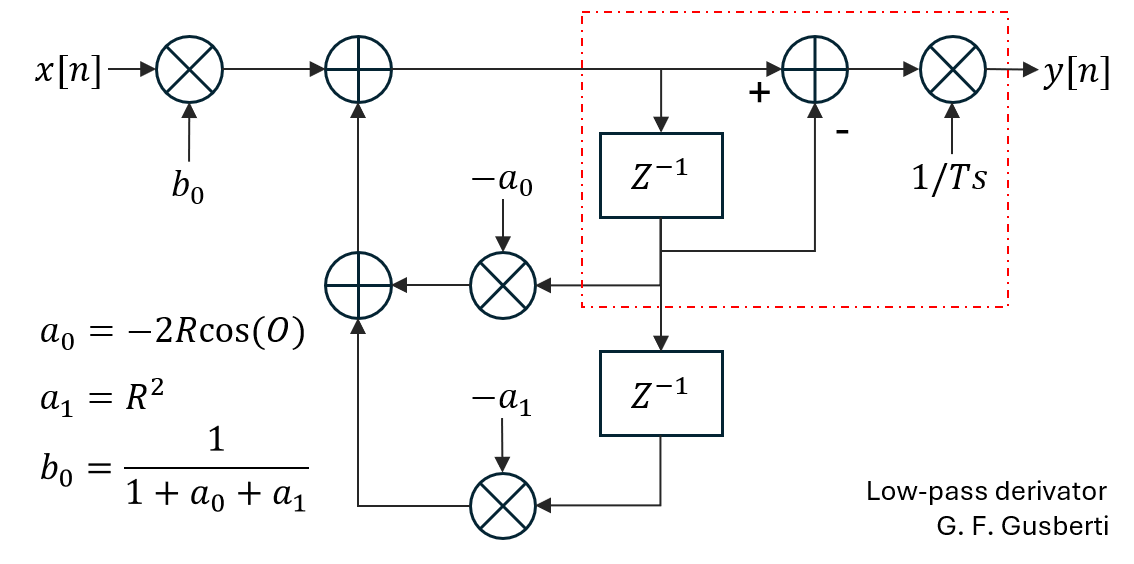
A first-difference derivator can be easily implemented in the output of the low-pass filter, as the direct-form I architecture conveniently presents the delay units on the right output side. Thus, the derivator is a simple difference between the output of the filter y[n] and its delayed version y[n - 1].
Term 1/Ts corrects the amplitude gain of the derivator, that follows directly from the base equation of a derivative df(x) = [f(x) - f(x - t)] / t. Figure 5 shows the implementation and, as the signal path is linear, it is possible to notice that the 1/Ts term can be combined with the input b0, replacing the b0 by b0/Ts and removing the 1/Ts gain completely.
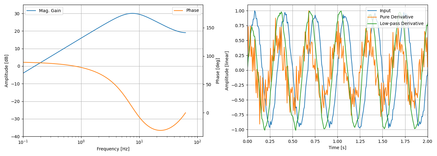
The proposed low-pass derivator presents a derivative magnitude gain and phase lead up to the resonance frequency of the low-pass structure, as seen in Figure 6. This creates a derivative action for the frequencies of interest, while reducing the noise-amplification effect of a derivator.
On the right of Figure 6, a time-domain comparison is shown, where the output amplitudes were normalized to the same level for a better qualitative analysis. The input signal (blue) has a small amount (~5% amplitude) of added Gaussian-noise, leading to a very noise output for a pure derivator (orange) - you can easily see how the noise dominates.
In the case of the low-pass derivator (green), the output signal is much cleaner and still presents the phase-lead needed for derivative controllers. Without filtering, all the noise of a pure derivator would pass through the controller reaching the plant, degrading the performance or even leading to an unusable closed-loop behavior.
It is important to notice that above the resonance frequency of the filter the low-pass derivator will introduce a phase lag, that can mess with the controller response. The engineer should understand this limitation and fall back to a 1st order low-pass filter when the introduced phase lag is a concern.
Conclusion
This article goes through the design procedure of a low-pass filter, by first composing a continuous-time transfer function - using its 2nd order geometrical properties in an intuitive way. By transposing the impulse-response to discrete-time using the impulse-invariant method, the weights for the proposed filter architecture are found.
The unusual requirements of using the damped frequency as a design parameter demonstrates the flexibility of the method, while maintaining the correctness of the 2nd-order transfer-function mathematics.
An application example is shown, where a first-difference discrete-time derivative is introduced at the output of the filter, utilizing an existing delay-unit that is provided by use of the direct-form I structure. The presented low-pass derivative has real utilization in practical control systems, allowing for enhanced stability and noise reduction.
References
[1]⠀https://www.dsprelated.com/freebooks/filters/Direct_Form_I.html
[2]⠀https://www.dsprelated.com/showarticle/120.php
[3]⠀https://www.dsprelated.com/freebooks/pasp/Impulse_Invariant_Method.html
[4]⠀https://www.dsprelated.com/showarticle/1341.php
[5]⠀https://controlsystemsacademy.com/0003/0003.html
